How to analyze thallium flux assay data

A step by step guide
In this short post, we’re going to walk you through how to get from raw to manuscript quality data when using thallium flux assays, including generating dose response curves and calculating EC50 values.

Step 1: Normalization (sometimes called baseline subtraction)

Start by defining your baseline (F0), which is the average fluorescence (RFU) for each individual well prior to stimulus* addition [*stimulus solutions typically include a compound of interest and thallium sulfate]. The number of data points to choose is going to depend on your read frequency, the time between the start of data collection and your stimulus addition, as well as the stability of your baseline. Although the baseline fluorescence for each well may vary slightly, the variation in the baseline for a given well should be relatively low. Typically the average of the first 5-15 data points is sufficient to generate a flat baseline. In this specific example, we collected 20 data points prior to stimulus addition. Since the baseline fluorescence is stable, choosing anywhere from 5 – 20 points should not have a significant impact on your normalized data. If you have a noisier baseline, you may consider averaging a larger number of data points.
Once you have calculated the F0 for each well, you divide every data point (F) in that curve by the F0 value. The end result of the normalization process is a kinetic trace (F/F0) where all baselines are equal to 1. This is an important correction to account for well to well variability caused by instrumentation, well position, slight differences in cell density between wells, or other factors (edge wells) that may cause certain wells to have a higher or lower fluorescence than others. Once all your data is normalized, trends that may not have been obvious when looking at your raw data should become more clear.

Step 2: Calculating the slope (or Vmax)

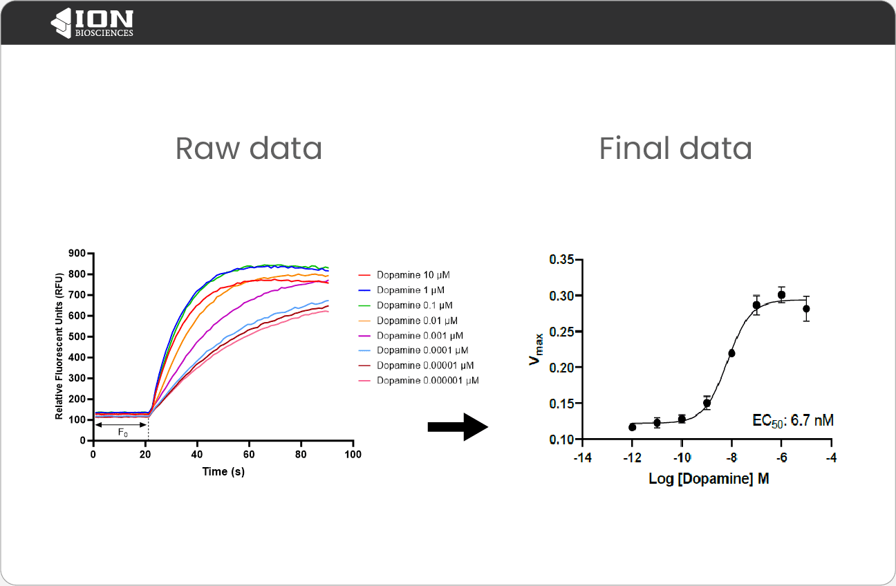
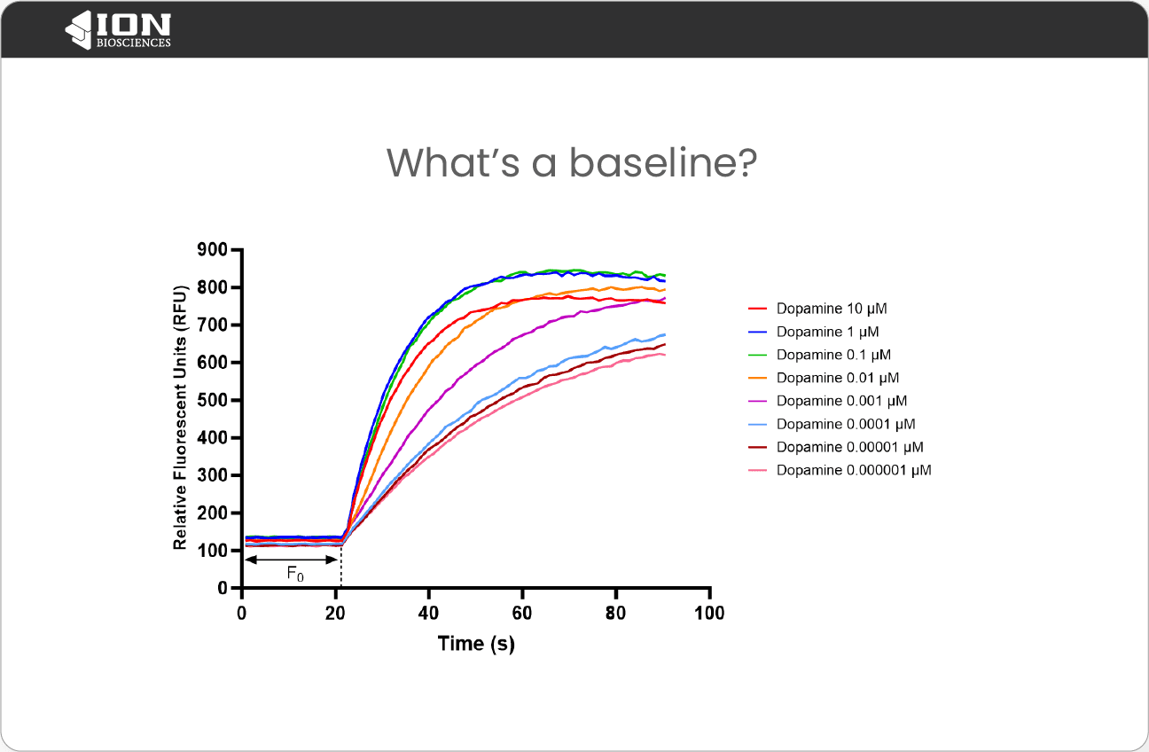
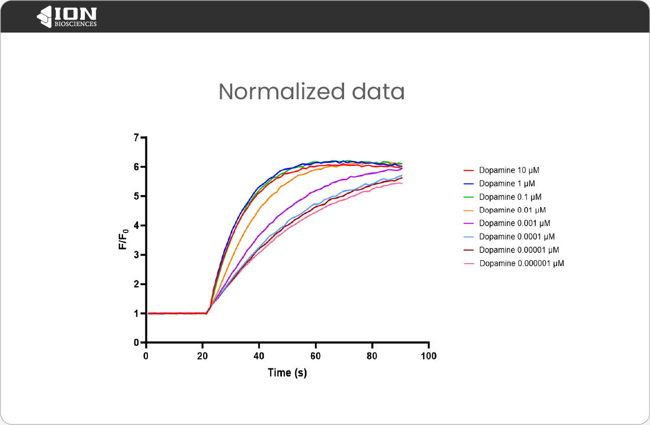
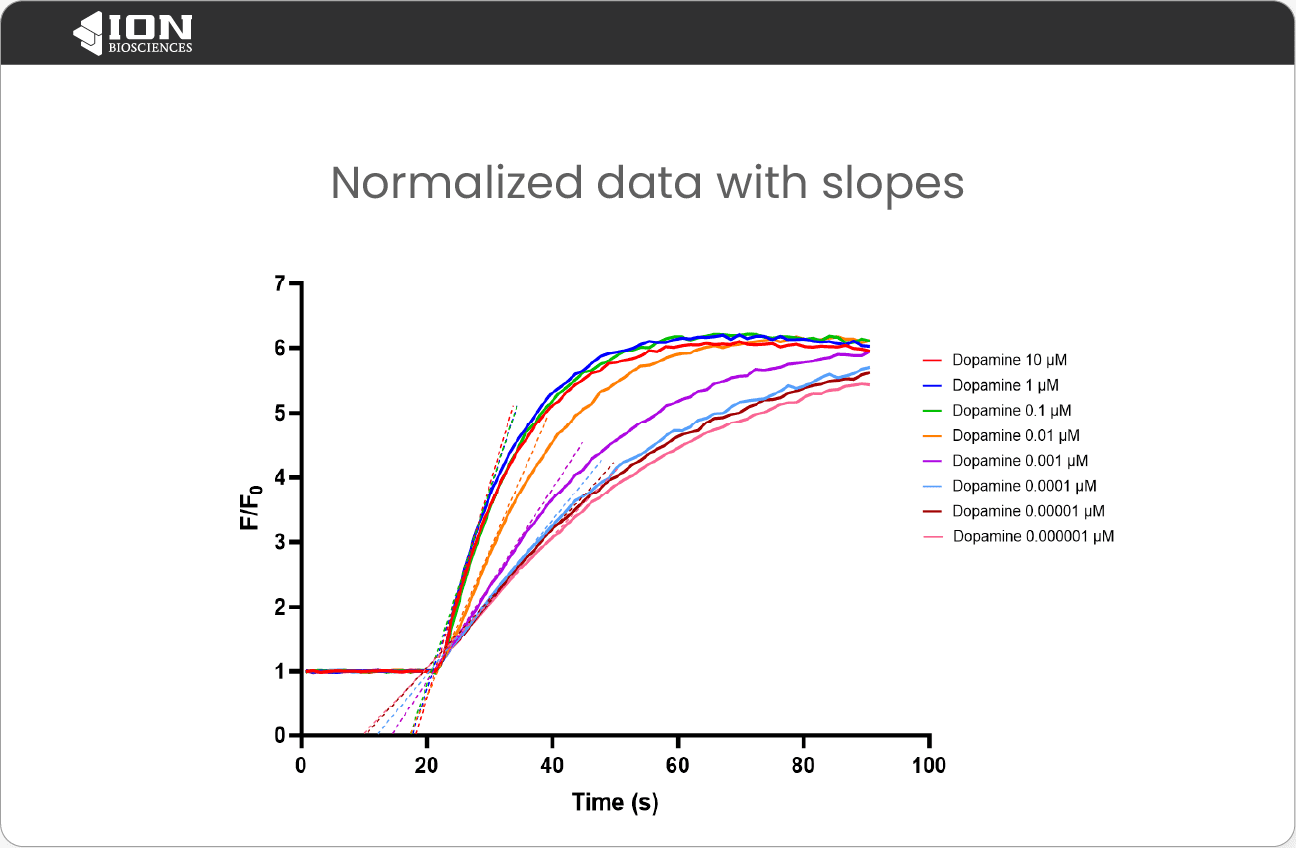
As the name suggests, thallium flux assays are designed to provide information about the activity of a potassium channel* based on the rate of thallium influx into your cells [*thallium flux assays can also be used for sodium channels, monovalent cation transporters, and Gi/o GPCRs.] The more open channels there are on a cell membrane, the faster thallium ions will enter into a cell. Alternatively, if channels are inhibited or blocked, the rate of thallium entry into a cell will be reduced. Therefore, to get an accurate measure of ion channel activity, the best approach is almost always to calculate the slope (or Vmax) of each normalized kinetic trace as soon after the addition of stimulus as possible.

To calculate the slope, you typically want to pick a range between 1-20 seconds after the addition of your stimulus solution and conduct a simple linear regression. The calculated slope is also referred to as Vmax (units/sec). As you can see in the plot below, the slope of F/F0 starts to decrease as intracellular thallium approaches tonic equilibrium. For this assay specifically, that downturn starts to occur within the first 15 seconds after stimulus addition, so we elected to calculate the slope using the first 10 data points after stimulus addition. A value in this range is usually sufficient for most assays, but may not be ideal if there are baseline anomalies from stimulus addition or if your influx rate is significantly faster. In these cases, choose a range that makes sense for your data.

Step 3: Using Vmax to generate a dose response curve

After Vmax has been calculated for each kinetic trace, create a plot of Vmax (y-axis) versus the log of your compound concentration (x-axis). The standard deviation for each concentration can be calculated from the Vmax values for replicates, and are usually used to generate y-axis error bars.

Step 4: Calculating an EC50 value

An EC50 value is defined as the concentration of your compound when it reaches 50% of its max effectiveness, and is indicative of a compound’s potency. A lower EC50 indicates a more potent compound, which is usually preferred in drug discovery. For inhibition assays, an IC50 is reported instead of an EC50.

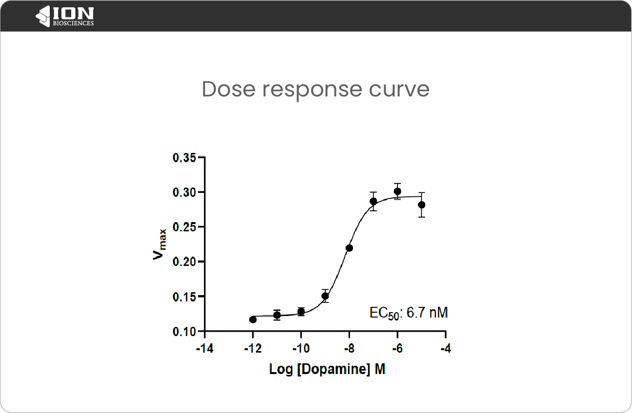
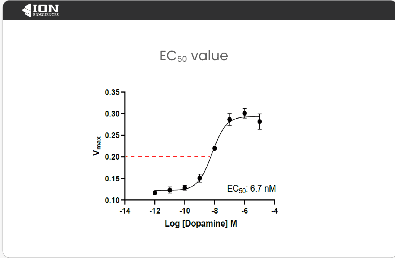
To calculate an EC50 value, apply a 4-parameter, non-linear fit with a variable slope to your dose response curve. Ensure you have chosen the right model for your assay. For example, we used log[agonist] vs. response since our compound increased the activity of our target at higher concentrations.

Fortunately, many software programs today make these steps incredibly simple and some will even do all the work for you. Be mindful that you are using the optimal settings for analyzing your data when relying on software to do all of the processing. If you have any questions, refer to this guide or reach out to us for additional troubleshooting tips.